
All of the code and software usage provided in this script was originally published by the authors (Benestan et al., 2016). Here, I am attempting to get the same results out using that analysis, explaining exactly what is meant by each part, and adding in some new visualizations to emphasize how you might extend this work for your own projects!
The authors include several, separate R scripts to analyze their data. It's up to use to construct the roadmap of how they put it all together.
codedir
├── scrip-rda-neutral.R
├── scrip-rda-selection-legendre.R
├── script_bayescan_laura.r
├── script-AEM.R
└── script-outflank.R
In addition, they provide several simplified text files that contain the environmental data they used for their analyses; in Environment.txt, for example, they list all of the minimum, maximum, and mean temperatures for each of the population localities that they examined, including total year values and just those for the summer.
After the authors used STACKS ("From the data set generated in that study, we developed a set of 13 688 filtered SNPs, which excluded SNPs that were not genotyped in at least 80% of the individuals and 70% of the locations, or did not show a minor allele frequency of at least 0.05 in all locations" (Benestan et al., 2016)) to generate their listing of 13,688 filtered SNPs, the next thing they did, per the paper, was:
used the software
outflank(Whitlock & Lotterhos 2015), which calculates a likelihood based on a trimmed distribution of FST values to infer the distribution of FST for neutral markers
The authors have provided an R script for this, so I'll just walk through each step of their script, which is essentially just using the software.
### Dowload libraries
install.packages("devtools")
library(devtools)

###Download source file
source("http://bioconductor.org/biocLite.R")
biocLite("qvalue")
install_github("whitlock/OutFLANK")

### Install OutFLANK package
library(qvalue)
library(OutFLANK)
Already we've run into a little hiccup: recent versions of R require that you use BiocManager. This is easy to fix. In addition to that, I prefer to use pacman (Rinker & Kurkiewicz, 2018) for downloading packages, a tool which simultaneously downloads and loads packages. I'll do this from now on, regardless of what the authors did in the paper.
pacman::p_load(devtools,qvalue,BiocManager)
BiocManager::install(c("qvalue"))
install_github("whitlock/OutFLANK")
library(OutFLANK)
pacman::p_load(vcfR)
# vcfFile <- read.vcfR("https://www.dropbox.com/s/yoy2i6a540zg8bf/13688snps-562individus.recode.vcf?dl=1")
# system(paste0("vcftools --vcf ", vcfFile, " --012 --out 13688snps-582ind.012.txt"))

# For some reason, the authors had the commands just listed out as they would be run in the console.
# To run these directory from R, we need to use `system`. I had to run this on a separate system, as it
# requires that you have `vcftools` installed locally.
system("vcftools --vcf ../../lobster-reproduction/data/lobster_download/13688snps-562individus.recode.vcf --012 --out ../../lobster-reproduction/data/13688snps-582ind.012.txt")
I think that a better way to do this is to use vcfR, which keeps everything within R, allows us to work straight out of Dropbox, and also doesn't involve odd matrix file formats and several intermediate files:
vcfFile <- read.vcfR("https://www.dropbox.com/s/yoy2i6a540zg8bf/13688snps-562individus.recode.vcf?dl=1")

## Create a genotype matrix using a vcfR utility.
genotypemat <- extract.gt(vcfFile, element = 'GT', as.numeric = FALSE)
# Any N/A values should be converted to 9s to prevent OutFLANK from complaining
genotypemat[is.na(genotypemat)] = 9

# Unlike vcftools, vcfR returns genotypes in 0/1 format, which requires that we convert them to just
# one numeric value.
mutatedgeno = data.frame(genotypemat)
for (c in 1:ncol(mutatedgeno)) {
    mutatedgeno[,c] = as.character(mutatedgeno[,c])
    for (r in 1:nrow(mutatedgeno)) {
        mutatedgeno[r,c] = sum(as.numeric(as.character(unlist(strsplit(as.character(mutatedgeno[r,c]), "/")))))
    }
}
head(mutatedgeno)
So now we have a matrix of genotypes without file I/O. Let's use the labels the authors provide to label the data and then feed the completed matrix into OutFLANK!
SNPmat <- mutatedgeno # instead of reading in output, we use what we produced above.
locusNames <- seq(from=1, to= 13688, by=1)
#popNames <- c(replicate(31,"ANT"), replicate(23,"BON"),replicate(34,"BOO"),replicate(23,"BRA"), replicate(36,"BRO"),replicate(34,"BUZ"),replicate(31,"CAN"),replicate(26,"CAP"),replicate(36,"CAR"), replicate(30,"GAS"),replicate(30,"LOB"),replicate(29,"MAL"),replicate(34,"MAR"),replicate(36,"OFF"),replicate(33,"RHO"),replicate(33,"SEA"),replicate(32,"SID"),replicate(18,"SJI"),replicate(33,"TRI"))
popNames <- strtrim(colnames(SNPmat), 3)
colnames(SNPmat) = popNames
rownames(SNPmat) = locusNames
SNPmat = t(SNPmat)
# Now we're working exclusively in OutFLANK (all code from 2015 paper!):
FstDataFrame <- MakeDiploidFSTMat(SNPmat,locusNames,popNames)

### Do the analysis with trim of 0.05
OFoutput <- OutFLANK(FstDataFrame, LeftTrimFraction=0.05,RightTrimFraction=0.05, Hmin=0.1, 19,qthreshold=0.05)
write.table(OFoutput, "Output_0.5_0.1_19pop.txt", quote=F)

### Do the analysis with trim of 0.1
OFoutput <- OutFLANK(FstDataFrame, LeftTrimFraction=0.1,RightTrimFraction=0.1, Hmin=0.1, 19,qthreshold=0.05)
write.table(OFoutput, "Output_0.5_0.1_19pop_without_trim.txt", quote=F)
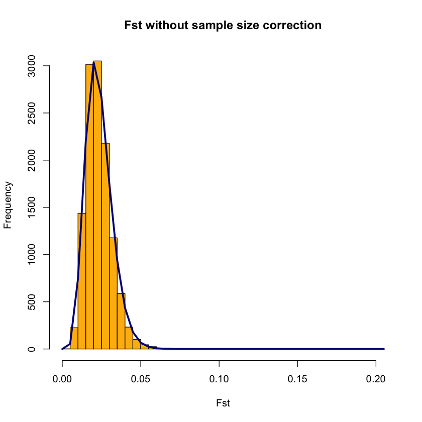
OutFLANKResultsPlotter(OFoutput, withOutliers = TRUE, NoCorr = TRUE, Hmin = 0.1, binwidth = 0.005, Zoom =FALSE, RightZoomFraction = 0.05, titletext = NULL)
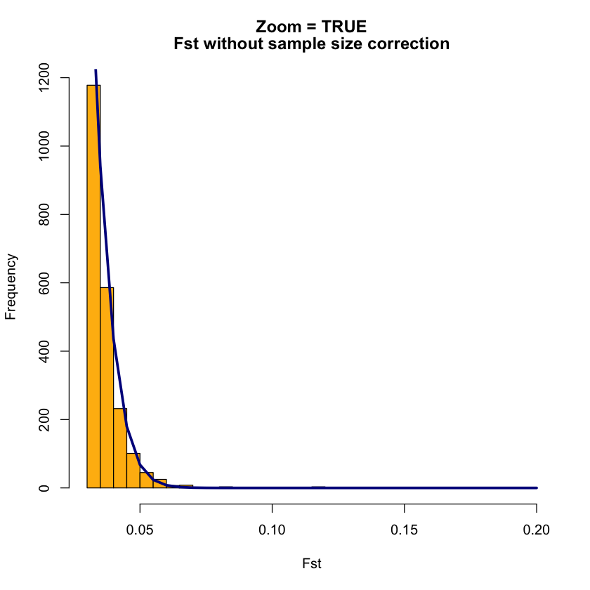
OutFLANKResultsPlotter(OFoutput, withOutliers = TRUE, NoCorr = TRUE, Hmin = 0.1, binwidth = 0.005, Zoom =TRUE, RightZoomFraction = 0.05, titletext = "Zoom = TRUE")
- Benestan, L., Quinn, B. K., Maaroufi, H., Laporte, M., Clark, F. K., Greenwood, S. J., … Bernatchez, L. (2016). Seascape genomics provides evidence for thermal adaptation and current-mediated population structure in American lobster (Homarus americanus). Molecular Ecology, 25(20), 5073–5092.
- Rinker, T. W., & Kurkiewicz, D. (2018). pacman: Package Management for R. Buffalo, New York. Retrieved from http://github.com/trinker/pacman